Class separation

library(biplotEZ)
#> Welcome to biplotEZ! 
#> This package is used to construct biplots 
#> Run ?biplot or vignette() for more information
#> 
#> Attaching package: 'biplotEZ'
#> The following object is masked from 'package:stats':
#> 
#>     biplot

This vignette deals with biplots for separating classes. Topics discussed are

• CVA (Canonical variate analysis) biplots
• AoD (Analysis of Distance) biplots
• Classification biplots

What is a CVA biplot

Consider a data matrix $\mathbf{X}:n \times p$ containing data on $n$ objects and $p$ variables. In addition, a vector $\mathbf{g}:n \times 1$ contains information on class membership of each observation. Let $G$ indicate the total number of classes. CVA is closely related to linear discriminant anlaysis, in that the $p$ variables are transformed to $p$ new variables, called canonical variates, such that the classes are optimally separated in the canonical space. By optimally separated, we mean maximising the between class variance, relative to the within class variance. This can be formulated as follows:

Let $\mathbf{G}:n \times G$ be an indicator matrix with $g_{ij} = 0$ unless observation $i$ belongs to class $j$ and then $g_{ij} = 1$. The matrix $\mathbf{G'G}$ is a diagonal matrix containing the number of observations per class on the diagonal. We can form the matrix of class means $\bar{\mathbf{X}}:G \times p = (\mathbf{G'G})^{-1} \mathbf{G'X}$. With the usual analysis of variance the total variance can be decomposed into a between class variance and within class variance:

$$\mathbf{T} = \mathbf{B} + \mathbf{W}$$

$$\mathbf{X'X} = \mathbf{\bar{\mathbf{X}}'C \bar{\mathbf{X}}} + \mathbf{X' [I - G(G'G)^{-1}C(G'G)^{-1}G'] X}$$

The default choice for the centring matrix $\mathbf{C = G'G}$ leads to the simplification

$$\mathbf{X'X} = \mathbf{\bar{\mathbf{X}}'G'G \bar{\mathbf{X}}} + \mathbf{X' [I - G(G'G)^{-1}G'] X}.$$

Other options are $\mathbf{C = I}$ and $\mathbf{C} = (\mathbf{I}_G - \frac{1}{G}\mathbf{11'})$. To find the canonical variates we want to maximise the ratio

$$\frac{\mathbf{m'Bm}}{\mathbf{m'Wm}}$$

subject to $\mathbf{m'Wm} = 1$. It can be shown that this leads to the following equivalent eigen equations:

$$\mathbf{W}^{-1}\mathbf{BM} = \mathbf{M \Lambda} \tag{1}$$

$$\mathbf{BM} = \mathbf{WM \Lambda}$$

$$(\mathbf{W}^{-\frac{1}{2}} \mathbf{B} \mathbf{W}^{-\frac{1}{2}}) \mathbf{M} = (\mathbf{W}^{-\frac{1}{2}} \mathbf{M}) \mathbf{\Lambda}$$

with $\mathbf{M'BM}= \mathbf{\Lambda}$ and $\mathbf{M'WM}= \mathbf{I}$.

Since the matrix $\mathbf{W}^{-\frac{1}{2}} \mathbf{B} \mathbf{W}^{-\frac{1}{2}}$ is symmetric and positive semi-definite the eigenvalues in the matrix $\mathbf{\Lambda}$ are positive and ordered. The rank of $\mathbf{B} = min(p, G-1)$ so that only the first $rank(\mathbf{B})$ eigenvalues are non-zero. We form the canonical variates with the transformation

$$\bar{\mathbf{Y}} = \bar{\mathbf{X}}\mathbf{M}.$$

To construct a 2D biplot, we plot the first two canonical variates $\bar{\mathbf{Z}} = \bar{\mathbf{X}}\mathbf{MJ}_2$ where $\mathbf{J}_2' = \begin{bmatrix} \mathbf{I}_2 & \mathbf{0} \end{bmatrix}$. We add the individual sample points with the same transformation

$$\mathbf{Z} = \mathbf{X}\mathbf{MJ}_2$$ where $$\mathbf{J}_2 = \begin{bmatrix} \mathbf{I}_2\\ \mathbf{0} \end{bmatrix}.$$ Interpolation of a new sample $\mathbf{x}^*:p \times 1$ follows as ${\mathbf{z}^*}':2 \times 1 ={\mathbf{x}^*}' \mathbf{MJ}_2$. Using the inverse transformation $\mathbf{x}' = \mathbf{y}'\mathbf{M}^{-1}$, all the points that will predict $\mu$ for variable $j$ will have the form

$$\mu = \mathbf{y}'\mathbf{M}^{-1} \mathbf{e}_j$$

where $\mathbf{e}_j$ is a vector of zeros with a one in position $j$. All the points in the 2D biplot that predict the value $\mu$ will have

$$\mu = \begin{bmatrix} z_1 & z_2 & 0 & \dots & 0\end{bmatrix}\mathbf{M}^{-1} \mathbf{e}_j$$

defining the prediction line as

$$\mu = \mathbf{z}_{\mu}' \mathbf{J}_2 \mathbf{M}^{-1} \mathbf{e}_j.$$

Writing $\mathbf{h}_{(j)} = \mathbf{J}_2 \mathbf{M}^{-1} \mathbf{e}_j$ the construction of biplot axes is similar to the discussion in the biplotEZ vignette for PCA biplots. The direction of the axis is given by $\mathbf{h}_{(j)}$. To find the intersection of the prediction line with $\mathbf{h}_{(j)}$ we note that $$\mathbf{z}'_{(\mu)}\mathbf{h}_{(j)} = \| \mathbf{z}_{(\mu)} \|^2 \| \mathbf{h}_{(j)} \|^2 cos(\mathbf{z}_{(\mu)},\mathbf{h}_{(j)}) = \| \mathbf{p} \|^2 \| \mathbf{h}_{(j)} \|^2$$ where $\mathbf{p}$ is the length of the orthogonal projection of $\mathbf{z}_{(\mu)}$ on $\mathbf{h}_{(j)}$.

Since $\mathbf{p}$ is along $\mathbf{h}_{(j)}$ we can write $\mathbf{p} = c\mathbf{h}_{(j)}$ and all points on the prediction line $\mu = \mathbf{z}'_{\mu}\mathbf{h}_{(j)}$ project on the same point $c_{\mu}\mathbf{h}_{(j)}$. We solve for $c_{\mu}$ from $$\mu = \mathbf{z}'_{\mu}\mathbf{h}_{(j)}=\| \mathbf{p} \|^2 \| \mathbf{h}_{(j)} \|^2 = \| c_{\mu}\mathbf{h}_{(j)} \|^2 \| \mathbf{h}_{(j)} \|^2$$

$$c_{\mu} = \frac{\mu}{\mathbf{h}_{(j)}'\mathbf{h}_{(j)}}.$$ If we select ‘nice’ scale markers $\tau_{1}, \tau_{2}, \cdots \tau_{k}$ for variable $j$, then $\tau_{h}-\bar{x}_j = \mu_{h}$ and positions of these scale markers on $\mathbf{h}_{(j)}$ are given by $p_{\mu_{1}}, p_{\mu_{2}}, \cdots p_{\mu_{k}}$ with $$p_{\mu_h} = c_{\mu_h}\mathbf{h}_{(j)} = \frac{\mu_h}{\mathbf{h}_{(j)}'\mathbf{h}_{(j)}}\mathbf{h}_{(j)}$$

$$= \frac{\mu_h}{\mathbf{e}_{(j)}' \mathbf{M'}^{-1} \mathbf{J} \mathbf{M}^{-1} \mathbf{e}_{(j)}}\ \mathbf{J}_2 \mathbf{M}^{-1} \mathbf{e}_{(j)}$$

with $$\mathbf{J} = \begin{bmatrix} \mathbf{I}_2 & \mathbf{0}\\ \mathbf{0} & \mathbf{0} \end{bmatrix}.$$

The function CVA()

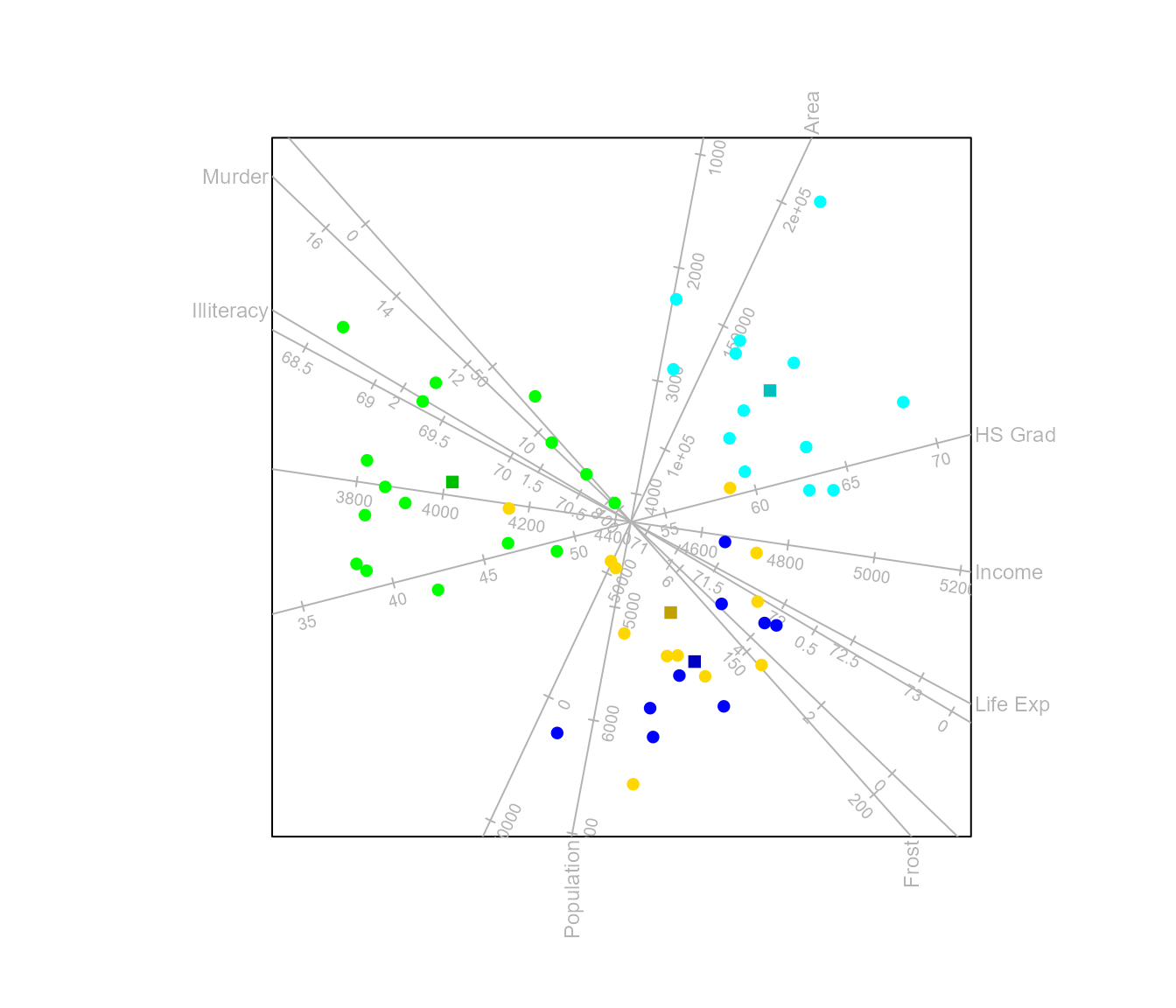
To obtain a CVA biplot of the state.x77 data set, optimally separating the classes according to state.region we call

biplot(state.x77) |> 
  CVA(classes = state.region) |> 
  plot()

Fitting $\alpha$-bags to the classes makes it easier to compare class overlap and separation. For a detailed discussion on $\alpha$-bags, see the biplotEZ vignette.

biplot(state.x77) |> CVA(classes = state.region) |> alpha.bags() |> 
  legend.type (bags = TRUE) |> 
  plot()
#> Computing 0.95 -bag for Northeast 
#> Computing 0.95 -bag for South 
#> Computing 0.95 -bag for North Central 
#> Computing 0.95 -bag for West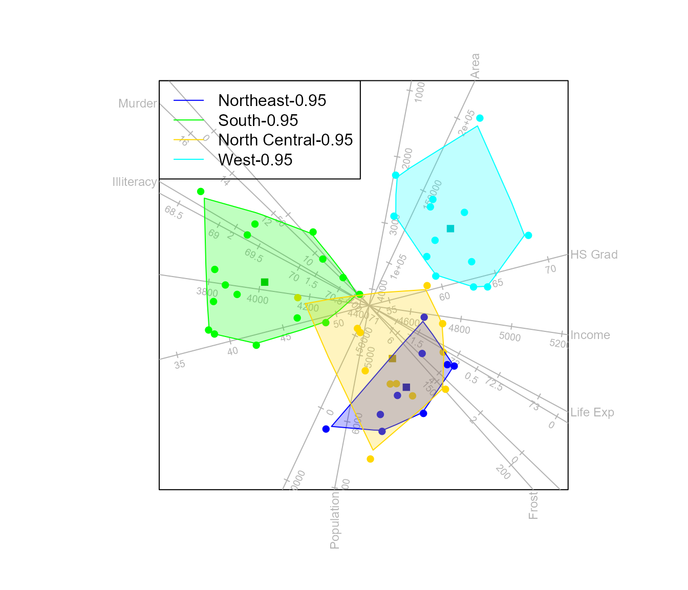

The function means()

This function controls the aesthetics of the class means in the biplot. The function accepts as first argument an object of class biplot where the aesthetics should be applied. Let us first construct a CVA biplot of the state.x77 data with samples optimally separated according to state.division.

biplot(state.x77, scaled = TRUE) |> 
  CVA(classes = state.division) |> 
  legend.type(means = TRUE) |> 
  plot()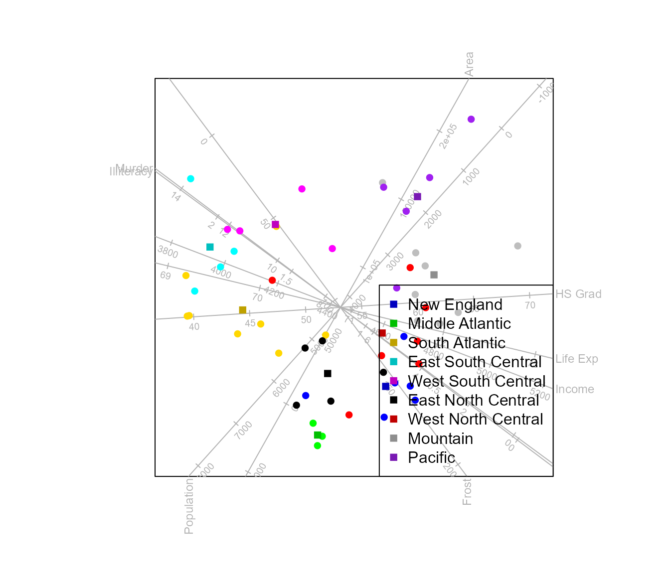

Instead of adding a legend, we can choose to label the class means. Furthermore, the colour of each class mean defaults to the colour of the samples. We wish to select a different colour and plotting character for the class means.

biplot(state.x77, scaled = TRUE) |> 
  CVA(classes = state.division) |> 
  means(label = TRUE, col = "olivedrab", pch = 15) |> 
  plot()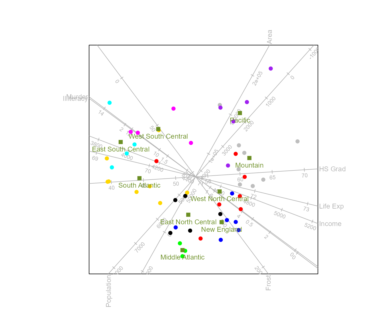

If we choose to only show the class means for the central states, the argument which is used either indicating the number(s) in the sequence of levels (which = 4:7), or as shown below, the levels themselves:

biplot(state.x77, scaled = TRUE) |> 
  CVA(classes = state.division) |> 
  means (which = c("West North Central", "West South Central", "East South Central", 
                     "East North Central"), label = TRUE) |>
  plot()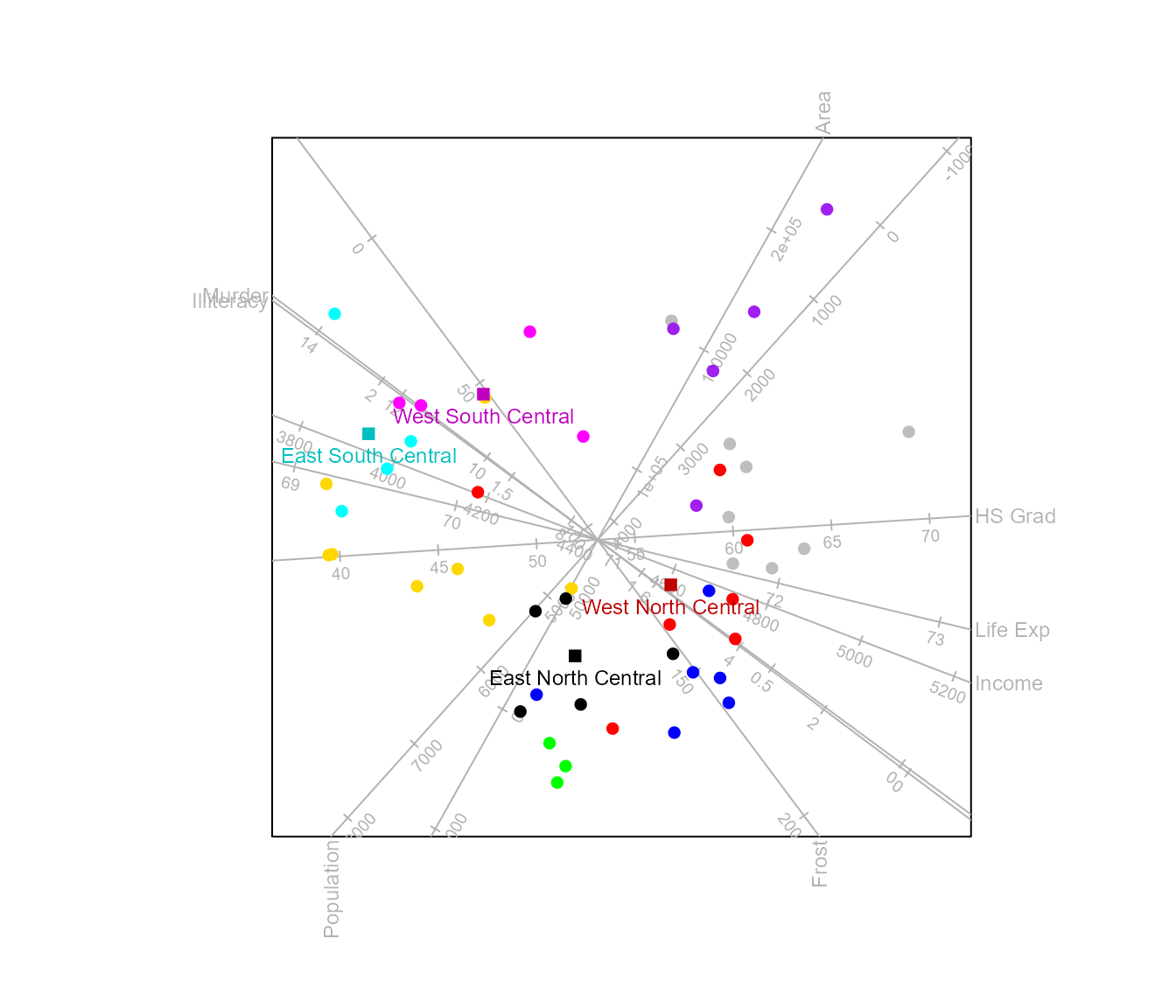

The size of the labels is controlled with label.cex which can be specified either as a single value (for all class means) or a vector indicating size values for each individual sample. The colour of the labels defaults to the colour(s) of the class means. However, individual label colours can be spesified with label.col, similar to label.cex as either a single value of a vector of length equal to the number of classes.

biplot(state.x77, scaled = TRUE) |> 
  CVA(classes = state.division) |> 
  means (col = "olivedrab", pch = 15, cex = 1.5,
         label = TRUE, label.col = c("blue","green","gold","cyan","magenta",
                                     "black","red","grey","purple")) |>
  plot()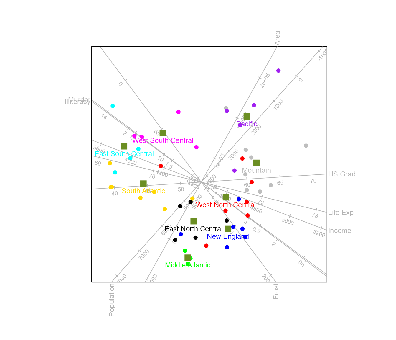

We can also make use of the functionality of the ggrepel package to place the labels.

biplot(state.x77, scaled = TRUE) |> 
  CVA(classes = state.division) |> 
  samples (label = "ggrepel", label.cex=0.65) |> 
  means (label = "ggrepel", label.cex=0.8) |> plot()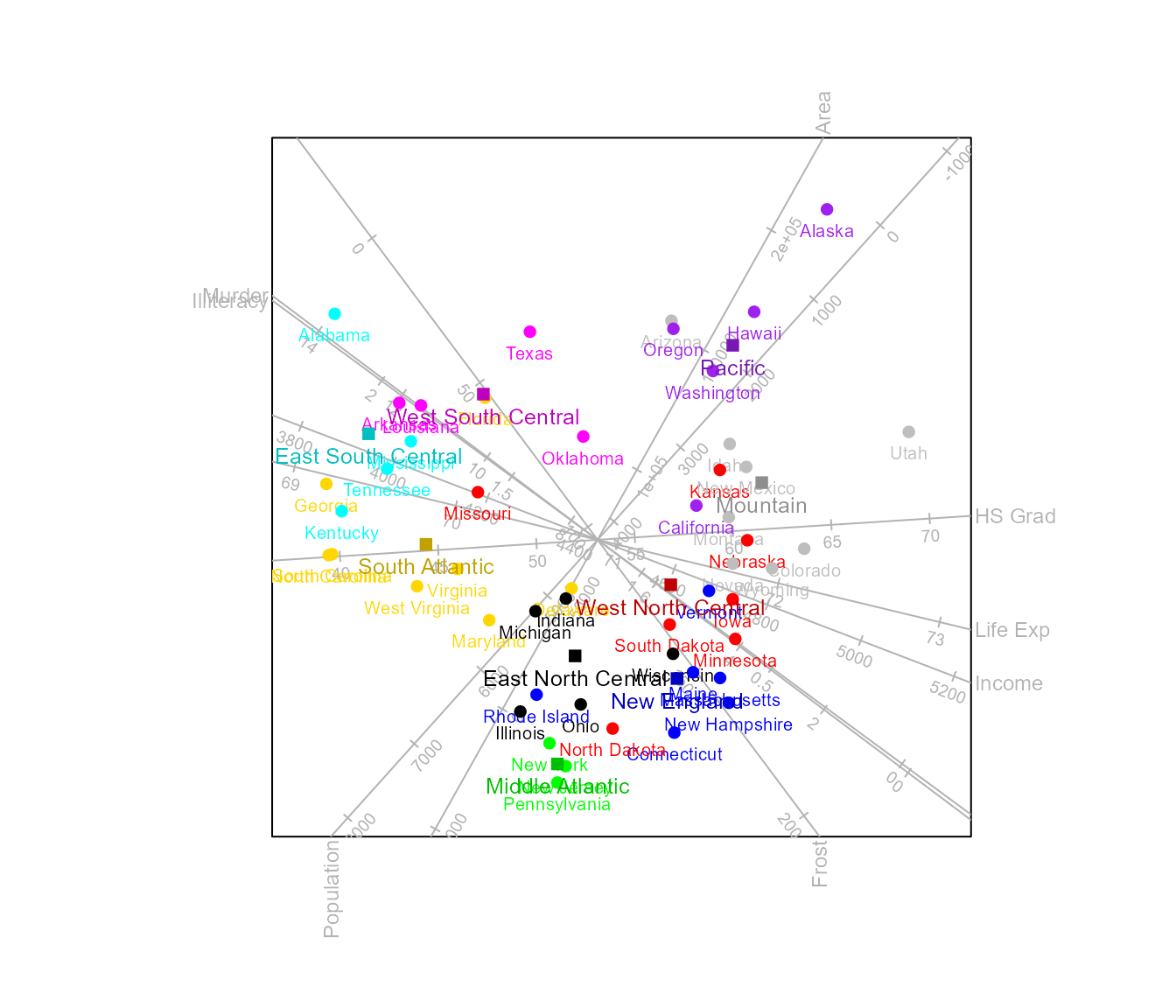

The function classify()

Classification regions can be added to the CVA biplot with the function classify(). The argument classify.regions must be set equal to TRUE to render the regions in the plot. Other arguments such as col, opacity and borders allows to change the aesthetics of the regions.

biplot(state.x77, scaled = TRUE) |> 
  CVA(classes = state.division) |>
  classify(classify.regions = TRUE,opacity = 0.2) |> 
  plot()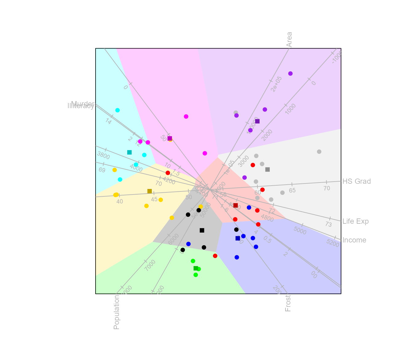

The functions fit.measures() and summary()

There is a number of fit measures that are specific to CVA biplots. The measures are computed with the function fit.measures() and the results are displayed by the function summary().

Canonical variate analysis can be considered as a transformation of the original variables to the canonical space followed by constructing a PCA biplot of canonical variables. The matrix of class means $\bar{\mathbf{X}} = (\mathbf{G'G})^{-1} \mathbf{G'X}$ is transformed to $\mathbf{\bar{X}L}$ where $\mathbf{L}$ is a non-singular matrix such that $\mathbf{LL'=W}^{-1}$. Pricipal component analysis finds the orthogonal matrix $\mathbf{V}$ such that

$$\mathbf{(L'\bar{X}'C\bar{X}L)V=V \Lambda}$$

where $\mathbf{M = LV}$ as defined in section 1. The predicted values for the class means is given by

$$\mathbf{\hat{\bar{X}}} = \mathbf{\bar{X}MJ}\mathbf{M}^{-1}.$$

Overall quality of fit

Based on the two-step process described above, there are two measures of quality of fit. The quality of the approximation of the canonical variables $\mathbf{\bar{X}L}$ in the $2$-dimensional display is given by

$$Quality (canonical \: variables) = \frac{tr(\mathbf{\Lambda J})}{tr(\mathbf{\Lambda)}}$$ and the quality of the approximation of the original variables $\mathbf{\bar{X}}$ in the 2D CVA biplot is given by

$$Quality (original \: variables) = \frac{tr(\mathbf{\Lambda J})}{tr(\mathbf{\Lambda)}}$$

Adequacy of representation of variables

The adequacy with which each of the variables is represented in the biplot is given by the elementwise ratios

$$Adequacy = \frac{diag(\mathbf{MJM'})}{diag(\mathbf{MM'})}.$$

Predictivity

Between class predictivity

The axis and class mean predictivities are defined in terms of the weighted class means.

Axis predictivity

The elementwise ratios for the predictivity of each of the axes are given by

$$axis \: predictivity = \frac{diag(\mathbf{\hat{\bar{X}}}'\mathbf{C\hat{\bar{X}}})}{diag(\mathbf{\bar{X}}'\mathbf{C\bar{X}})}.$$

Class predictivity

Similarly for each of the class means the elementwise ratio is computed from

$$class \: predictivity = \frac{diag(\mathbf{C}^{\frac{1}{2}}\mathbf{\hat{\bar{X}}}'\mathbf{W^{-1}}\mathbf{\hat{\bar{X}}}\mathbf{C}^{\frac{1}{2}})}{diag(\mathbf{C}^{\frac{1}{2}}\mathbf{\bar{X}}'\mathbf{W^{-1}}\mathbf{\bar{X}}\mathbf{C}^{\frac{1}{2}})}.$$

Within class predictivity

We define the matrix of samples as deviations from their class means as

$$(\mathbf{I-H})\mathbf{X}=(\mathbf{I}_n-\mathbf{G}(\mathbf{G'G})^{-1}\mathbf{G}')\mathbf{X}$$

where $\mathbf{H} = \mathbf{G}(\mathbf{G'G})^{-1}\mathbf{G}'$.

Within class axis predictivity

The within class axis predictivity is computed as the elementwise ratios

$$within \: class \: axis \: predictivity = \frac{diag(\mathbf{\hat{X}}'(\mathbf{I-H)\hat{X}})}{diag(\mathbf{X}'(\mathbf{I-H)X})}.$$

Within class sample predictivity

Unlike PCA biplots, sample predictivity for CVA biplots are computed for the observations expressed as deviations from their class means. The elementwise ratios is obtained from

$$within \: class \: axis \: predictivity = \frac{diag(\mathbf{(I-H)\hat{X}}\mathbf{W}^{-1}\mathbf{\hat{X}'(I-H)})}{diag(\mathbf{(I-H)X}\mathbf{W}^{-1}\mathbf{X'(I-H)})}.$$ To display the fit measures, we create a biplot object with the measures added by the function fit.measures() and call summary().

obj <- biplot(state.x77, scaled = TRUE) |> 
       CVA(classes = state.division) |> 
       fit.measures() |>
       plot()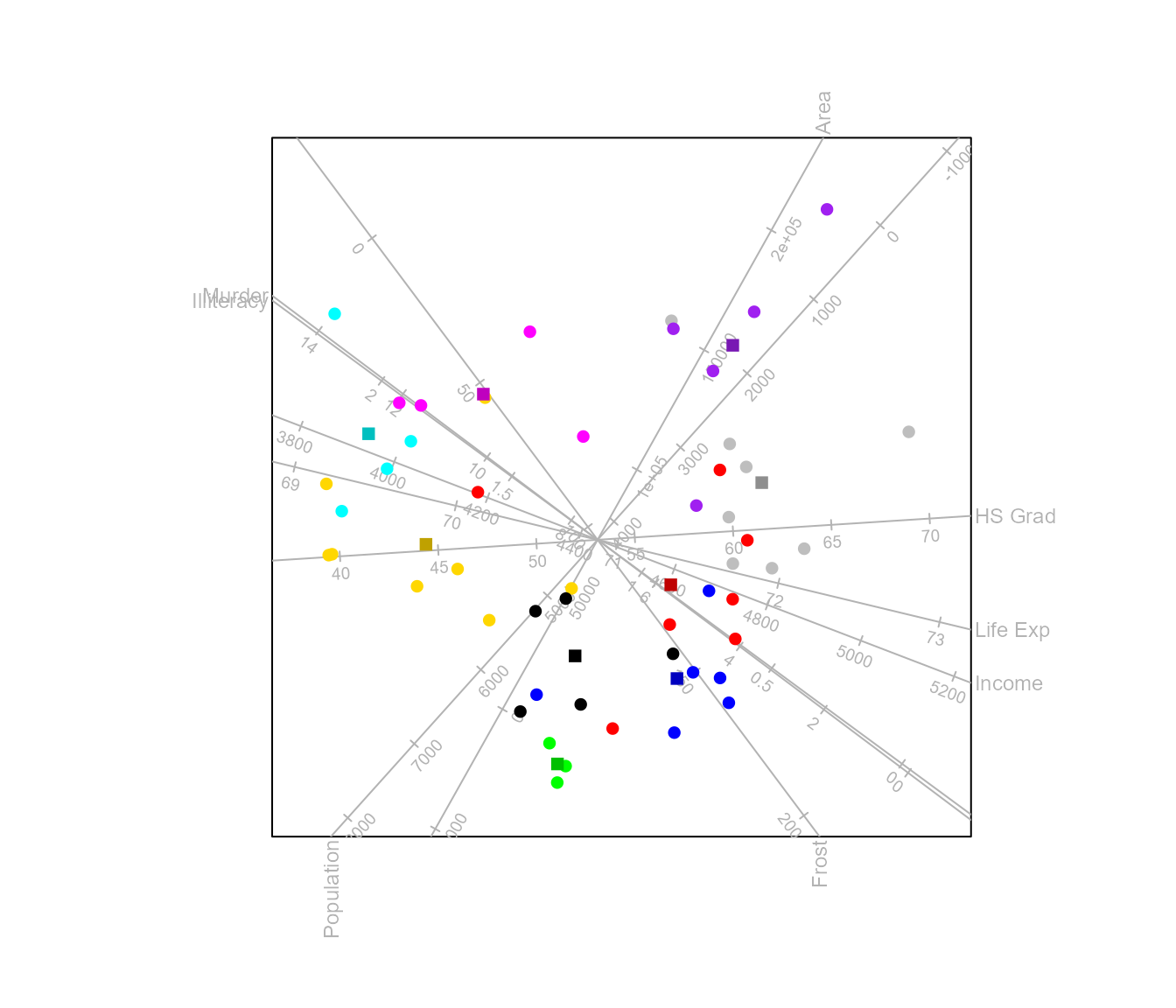

summary (obj)
#> Object of class biplot, based on 50 samples and 8 variables.
#> 8 numeric variables.
#> 9 classes: New England Middle Atlantic South Atlantic East South Central West South Central East North Central West North Central Mountain Pacific 
#> 
#> Quality of fit of canonical variables in 2 dimension(s) = 70.7% 
#> Quality of fit of original variables in 2 dimension(s) = 70.5% 
#> Adequacy of variables in 2 dimension(s):
#> Population     Income Illiteracy   Life Exp     Murder    HS Grad      Frost 
#> 0.41716176 0.15621549 0.16136381 0.09759664 0.19426796 0.55332679 0.50497634 
#>       Area 
#> 0.40661470 
#> Axis predictivity in 2 dimension(s):
#> Population     Income Illiteracy   Life Exp     Murder    HS Grad      Frost 
#>  0.1859124  0.4019427  0.8195756  0.6925389  0.7685373  0.9506355  0.7819324 
#>       Area 
#>  0.8458143 
#> Class predictivity in 2 dimension(s):
#>        New England    Middle Atlantic     South Atlantic East South Central 
#>          0.7922047          0.6570417          0.8191791          0.8777759 
#> West South Central East North Central West North Central           Mountain 
#>          0.7416085          0.6370315          0.3265978          0.6825966 
#>            Pacific 
#>          0.6700194 
#> Within class axis predictivity in 2 dimension(s):
#> Population     Income Illiteracy   Life Exp     Murder    HS Grad      Frost 
#> 0.04212318 0.09357501 0.25675620 0.19900223 0.29474972 0.75215233 0.31027358 
#>       Area 
#> 0.12741853 
#> Within class sample predictivity in 2 dimension(s):
#>        Alabama         Alaska        Arizona       Arkansas     California 
#>    0.722548912    0.163442379    0.333341120    0.268976273    0.229139828 
#>       Colorado    Connecticut       Delaware        Florida        Georgia 
#>    0.264963758    0.082284385    0.593415987    0.461070888    0.636531435 
#>         Hawaii          Idaho       Illinois        Indiana           Iowa 
#>    0.015640188    0.113711473    0.338612599    0.389208196    0.507060148 
#>         Kansas       Kentucky      Louisiana          Maine       Maryland 
#>    0.784831952    0.314119027    0.078465054    0.008388471    0.306141816 
#>  Massachusetts       Michigan      Minnesota    Mississippi       Missouri 
#>    0.076563044    0.218470793    0.645446212    0.046129058    0.710971640 
#>        Montana       Nebraska         Nevada  New Hampshire     New Jersey 
#>    0.086279776    0.810374638    0.090490164    0.298187909    0.003496353 
#>     New Mexico       New York North Carolina   North Dakota           Ohio 
#>    0.007134343    0.024268121    0.422776032    0.446240464    0.277262145 
#>       Oklahoma         Oregon   Pennsylvania   Rhode Island South Carolina 
#>    0.450104680    0.108636860    0.033945796    0.415029328    0.261568299 
#>   South Dakota      Tennessee          Texas           Utah        Vermont 
#>    0.134881180    0.247921823    0.110537439    0.500454605    0.159941068 
#>       Virginia     Washington  West Virginia      Wisconsin        Wyoming 
#>    0.310439564    0.030877305    0.066303623    0.295499472    0.474458397

The call to biplot(), CVA() and fit.measures() is required to (a) create an object of class biplot, (b) extend the object to class CVA and (c) compute the fit measures. The call to the function plot() is optional. It is further possible to select which fit measures to display in the summary() function where all measures default to TRUE.

obj <- biplot(state.x77, scaled = TRUE) |> 
       CVA(classes = state.region) |> 
       fit.measures()
summary (obj, adequacy = FALSE, within.class.axis.predictivity = FALSE,
         within.class.sample.predictivity = FALSE)
#> Object of class biplot, based on 50 samples and 8 variables.
#> 8 numeric variables.
#> 4 classes: Northeast South North Central West 
#> 
#> Quality of fit of canonical variables in 2 dimension(s) = 91.9% 
#> Quality of fit of original variables in 2 dimension(s) = 95.3% 
#> Axis predictivity in 2 dimension(s):
#> Population     Income Illiteracy   Life Exp     Murder    HS Grad      Frost 
#>  0.9873763  0.9848608  0.8757913  0.9050208  0.9955088  0.9970346  0.9558192 
#>       Area 
#>  0.9344651 
#> Class predictivity in 2 dimension(s):
#>     Northeast         South North Central          West 
#>     0.8031465     0.9985089     0.6449906     0.9988469

Additional CVA dimensions

It was mentioned that the eigen equation (1) has $min(p, G-1)$ non-zero eigenvalues. This implies that the CVA biplot for $G=2$ groups, reduces to a single dimension. If we write

$$\mathbf{M} = \begin{bmatrix} \mathbf{m}_1 & \mathbf{M}^* \end{bmatrix}$$ the columns of $\mathbf{M}^*$ forms a basis for the orthogonal complement of the canonical space defined by $\mathbf{m}$_1. The argument low.dim determines how to uniquely define the second and third dimensions. By default low.dim = "sample.opt" which selects the dimensions by minimising total squared reconstruction error for samples.

The representation of the canonical variates $\bar{\mathbf{Z}} = \bar{\mathbf{X}}\mathbf{m}_1$ are exact in the first dimension, but not the representation of the individual samples ${\mathbf{Z}} = {\mathbf{X}}\mathbf{m}_1$. If we define $\mathbf{\hat{X}} = \mathbf{XMJ}\mathbf{M}^{-1}$ with $\mathbf{J}$ a square matrix of zeros except for a $1$ in the first diagonal position, then the total square reconstruction error for samples is given by

$$TSRES = tr{(\mathbf{X}-\mathbf{\hat{X}})'(\mathbf{X}-\mathbf{\hat{X}})}.$$ Define $$\mathbf{M}^{-1} = \begin{bmatrix} \mathbf{M}^{(1)}:(G-1) \times p \\ \mathbf{M}^{(2)}: (p-G+1) \times p \end{bmatrix}$$

then $TSRES$ is minimised when

$$\mathbf{M}^{opt} = \begin{bmatrix} \mathbf{M}_1 & \mathbf{M}^*\mathbf{V} \end{bmatrix}$$

where where $\mathbf{V}$ is the matrix of right singular vectors of $\mathbf{M}^{(2)}\mathbf{M}^{(2)'}$.

state.2group <- ifelse(state.division == "New England" | 
                       state.division == "Middle Atlantic"  |
                       state.division == "South Atlantic" |
                       state.division == "Pacific",
                       "Coastal", "Central")
biplot (state.x77) |> CVA (state.2group) |> legend.type(means=TRUE) |> plot()
#> Warning in CVA.biplot(biplot(state.x77), state.2group): The dimension of the
#> canonical space < dim.biplot sample.opt method used for additional
#> dimension(s).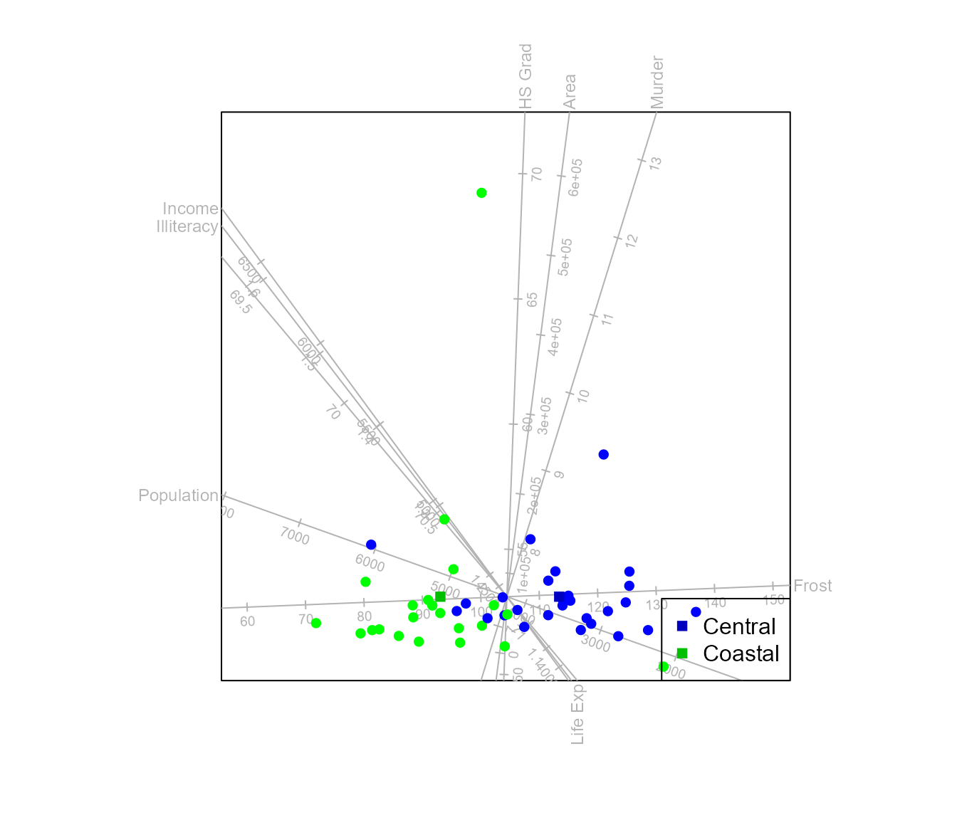

le Roux and Gardner-Lubbe (2024) discuss an alternative method for obtaining additional dimensions. When assuming underlying normal distributions, the Bhattacharyya distance can be optimised. This method is specific to the two class case and cannot be utilised to find a third dimension in a 3D CVA biplot with three classes.

biplot (state.x77) |> CVA (state.2group, low.dim="Bha") |> legend.type(means=TRUE) |> plot()
#> Warning in CVA.biplot(biplot(state.x77), state.2group, low.dim = "Bha"): The
#> dimension of the canonical space < dim.biplot Bhattacharyya.dist method used
#> for additional dimension(s).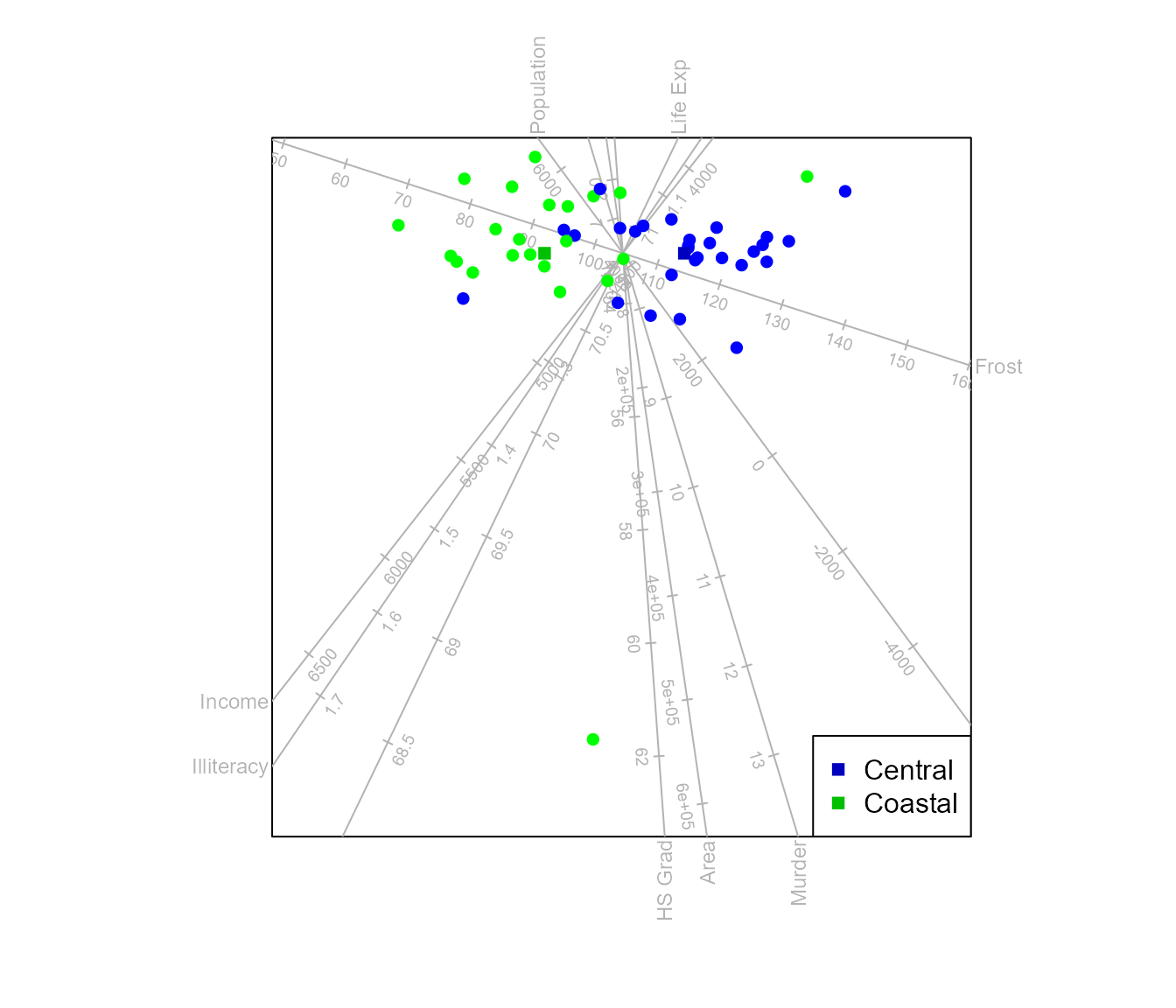

Analysis of Distance (AoD)

Similar to the variance decomposition in CVA, analysis of distance decomposes the total sum of squared distances into a sum of squared distances between class means component and a sum of squared distances within classes component.

Consider any Euclidean embeddable distance metric $\psi_{ij}=\psi(\mathbf{x}_i,\mathbf{x}_j)$. For a Euclidean embeddable metric it is possible to find high dimensional coordinates $\mathbf{y}_i$ and $\mathbf{y}_j$ such that the Euclidean distance between $\mathbf{y}_i$ and $\mathbf{y}_j$ is equal to $\psi_{ij}$. Let the matrix $\mathbf{\tilde\Psi}$ contain the values $-\frac{1}2{}\psi_{ij}^2$ and similarly $\mathbf{\tilde\Delta}$ the values $-\frac{1}2{}\delta_{hk}^2$ where $\delta_{hk}$ represent the distance between class means $h$ and $k$.

$$\mathbf{T} = \mathbf{B} + \mathbf{W}$$

$$\mathbf{1'\tilde\Psi1} = \mathbf{n'\tilde\Delta n} + \sum_{k=1}^{G} \frac{n}{n_k} \mathbf{g}_k'\mathbf{\tilde\Psi}\mathbf{g}_k$$ where $\mathbf{n}=\mathbf{(G'G)1}$. Thus, AoD differs from CVA in allowing any Euclidean embeddable measure of inter-class distance. As with CVA, these distances may be represented in maps with point representing the class means, supplemented by additional points representing the within-group variation. Principal coordinate analysis is performed, only on the $G \times G$ matrix $\mathbf{\tilde\Delta}$.

biplot(state.x77, scaled = TRUE) |> AoD(classes = state.region) |> plot()

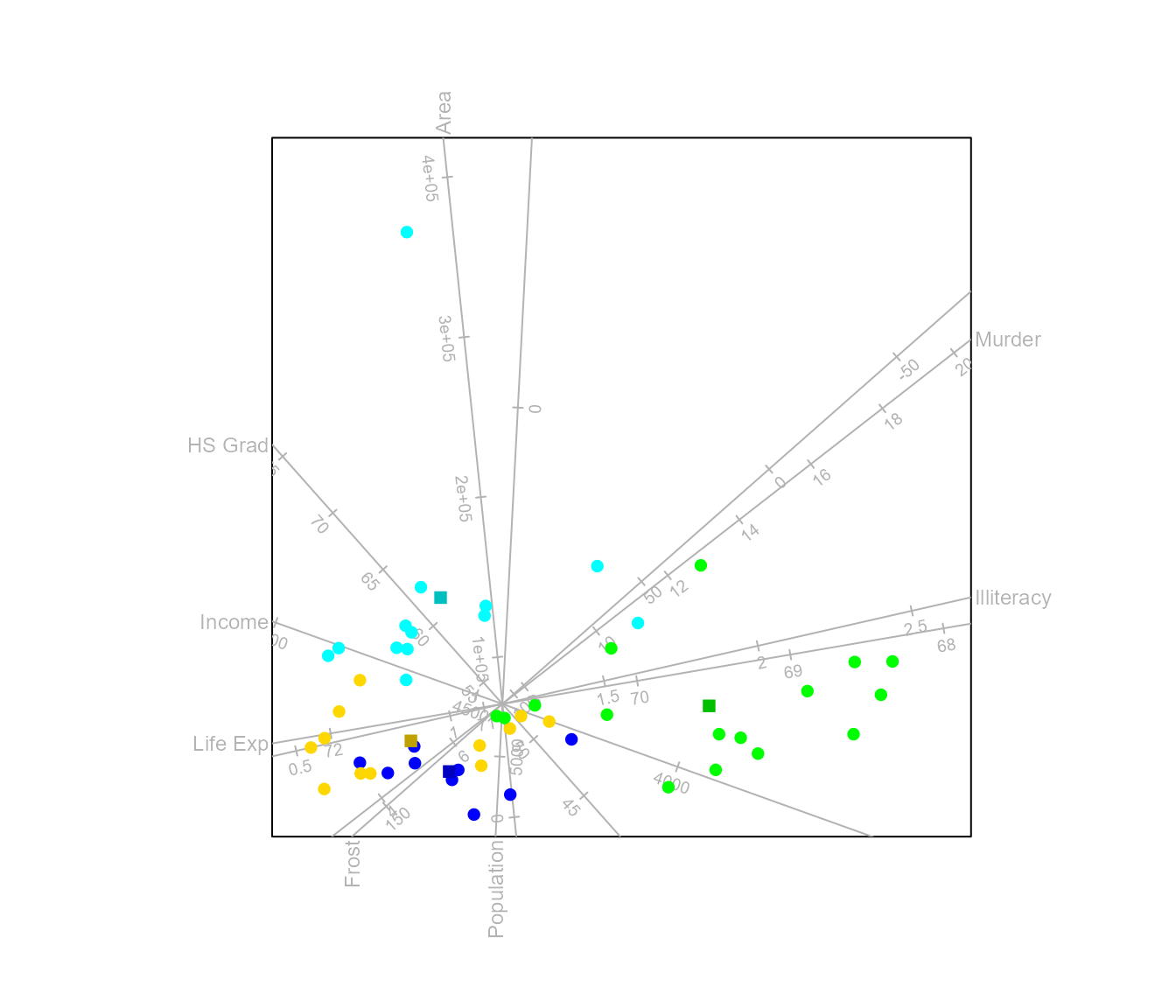
By default linear regression biplot axes are fitted to the plot. Alternatively, spline axes can be constructed.

biplot(state.x77, scaled = TRUE) |> AoD(classes = state.region, axes = "splines") |> plot()
#> Warning: The ggplot2 engine does not yet support spline axes; falling back to
#> base graphics.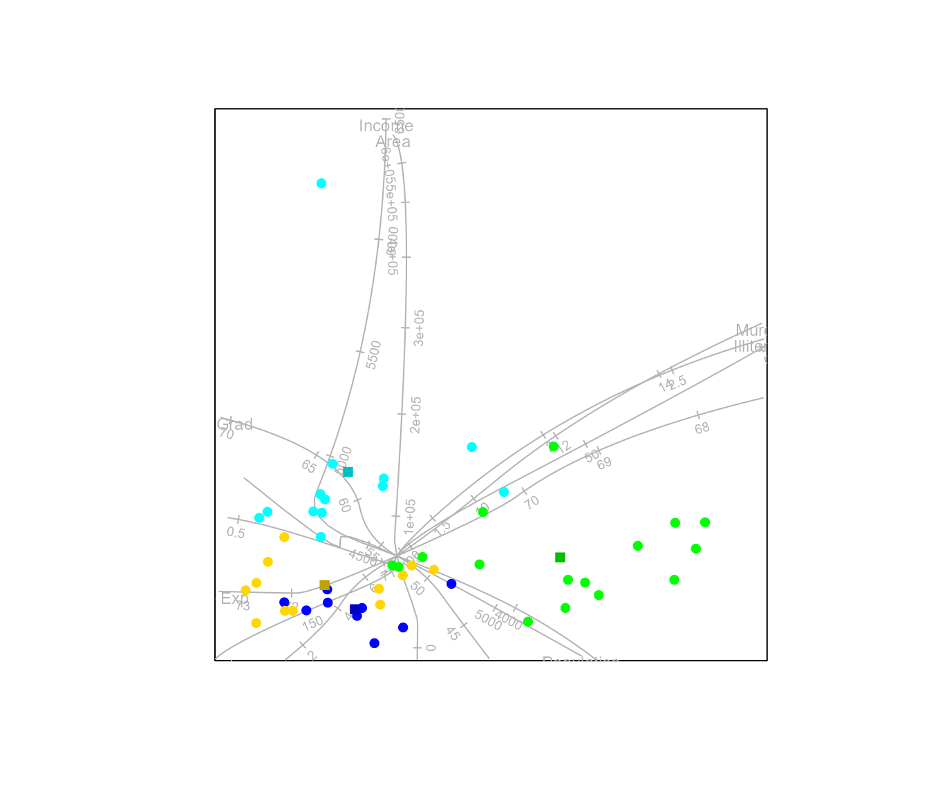

#> Calculating spline axis for variable 1 
#> Calculating spline axis for variable 2 
#> Calculating spline axis for variable 3 
#> Calculating spline axis for variable 4 
#> Calculating spline axis for variable 5 
#> Calculating spline axis for variable 6 
#> Calculating spline axis for variable 7 
#> Calculating spline axis for variable 8

As an illustration of a Euclidean embeddable distance metric, other than Euclidean distance itself, we can construct an AoD biplot with the square root of the Manhattan distance.

biplot(state.x77, scaled = TRUE) |> 
  AoD(classes = state.region, axes = "splines", dist.func=sqrtManhattan) |> plot()
#> Warning: The ggplot2 engine does not yet support spline axes; falling back to
#> base graphics.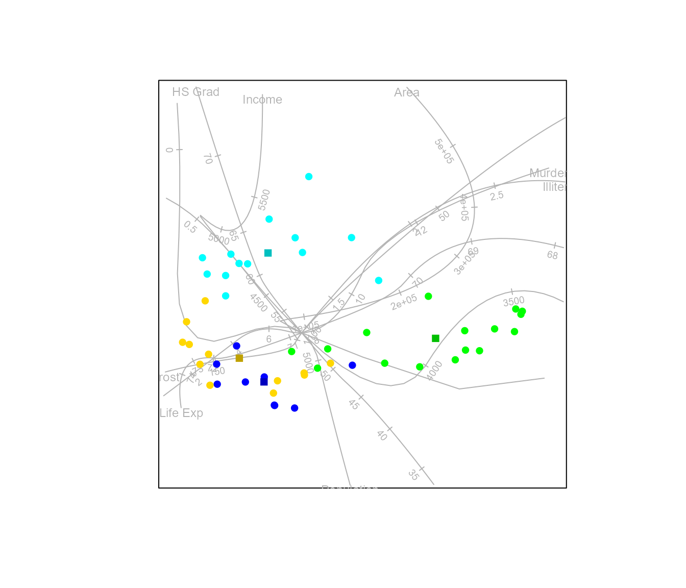

#> Calculating spline axis for variable 1 
#> Calculating spline axis for variable 2 
#> Calculating spline axis for variable 3 
#> Calculating spline axis for variable 4 
#> Calculating spline axis for variable 5 
#> Calculating spline axis for variable 6 
#> Calculating spline axis for variable 7 
#> Calculating spline axis for variable 8

References

le Roux, N. J, and S. Gardner-Lubbe. 2024. “A Two-Group Canonical Variate Analysis Biplot for an Optimal Display of Bothmeans and Cases.” Advances in Data Analysis and Classification.